数値微分

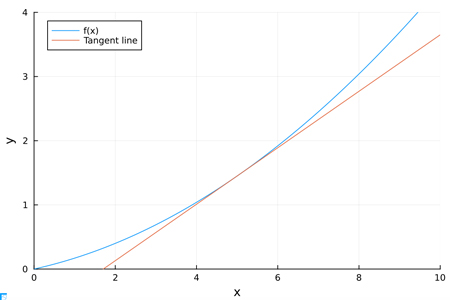
数値微分の値を傾きとする直線をJuliaを用いてグラフにする.

using Plots

function numerical_diff(f, x)
    h = 1e-4
    return (f(x+h) - f(x-h)) / (2*h)
end

#1変数関数を定義
function function_1v(x)
    return 0.03*x^2 + 0.14*x
end

function tangent_line(f, x)
    slope = numerical_diff(f, x)
    y = f(x) - slope*x
    return slope, y
end

#x 切片の計算を別の関数 x_intercept にカプセル化することにより,
#コードの可読性が高まる
function x_intercept(slope, intercept)
    return -intercept / slope
end

#0から10まで0.1刻みの配列を作成
x = 0:0.1:10.0

#function_1v関数をベクトル化し,xの各要素に適用
#.を使うことにより,関数をベクトル化
y1 = function_1v.(x)

#tangent_line関数を呼び出し,function_1vのx = 5における接線の傾きと切片を取得
slope, intercept = tangent_line(function_1v, 5)

#slopeとinterceptから接線の方程式y = mx + bを計算
#.*と.+は配列の要素ごとの乗算と加算を行うブロードキャスト演算
y2 = slope.*x .+ intercept

#新しいプロットを作成し,そのプロットハンドルを p に割り当て
p = plot(x, y1, label="f(x)", xlabel="x", ylabel="y", xlim=(0, 10), ylim=(0, 4))

#既存のプロットハンドル p に対して,新しいプロットを追加
plot!(p, x, y2, label="Tangent line")

# x切片の計算
x_int = x_intercept(slope, intercept)
# 数値微分の値を出力
numerical_diff_val = numerical_diff(function_1, 5)
println("数値微分の結果 = $numerical_diff_val")
println("x切片の座標: ($x_int, 0)")

#グラフを表示
display(p)

アウトプットは以下のようになる.

数値微分の結果 = 0.4399999999982196
x切片の座標: (1.7045454545321195, 0)

Mathematics is the language with which God has written the universe.